Phase 2 submission
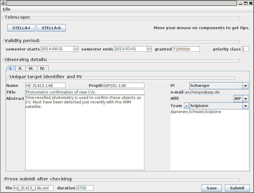
After successfully launching the target preparation tool, a GUI similar to the window to the right will pop up. Pre-selected fields will be grayed-out. They have been set following your proposal and cannot be changed. This normally applies to the Validity period [1] , and the time granted [2] to your proposal. The priority class [3] is assigned depending on how time-crucial the picking of the target is: higher prioirty classes mean a higher likelihood of selection.
Once you filled all the information, the duration [4] field holds an estimated of the time required for a single observation of the target. Press Save to save your work for later continuation, or Submit to finally create the observing block and submit it to the operator - whatch out for a pop-up infomraing that the target has been successfully created. Once the target has been uploaded, you will receive an e-mail summarizing the main contratints of the target. Immediately after the upload, the target is available for the robotic schedule. As a final manual check is still required, up to 72 hour may pass from submission to actual upload.
Target preparation tool overview
Only two fields normally remain to be filled on that page, everything else is already pre-filled once your proposal has been accepted. The most critical information is in the Name fields, which must be a unique identifier for your target. It is recommended to put here a classical object name, followed by your initials and/or the target semester. Note that using an already used name is forbidden and will result in an error message.
The second important field is the list of your team, i.e., users that may retrieve the data (only the PI may upload targets, though). Select the user to add to your team from the drop-down box and hit plus to add her. Hit plus again to remove him again.
Footnotes
| [1] | The target will only be active during this semester. |
| [2] | This is the time granted for this proposal. It is stated in ms. |
| [3] | Higher numbers mean higher priorities. Levels-off the maximum priority a target can achieve. |
| [4] | From the sequence and exposure time, a duration for one target execution is estimated. This duration is used in the Constraints section and also during .. scheduling to check for intervening high-priority targets. |
A single observing block
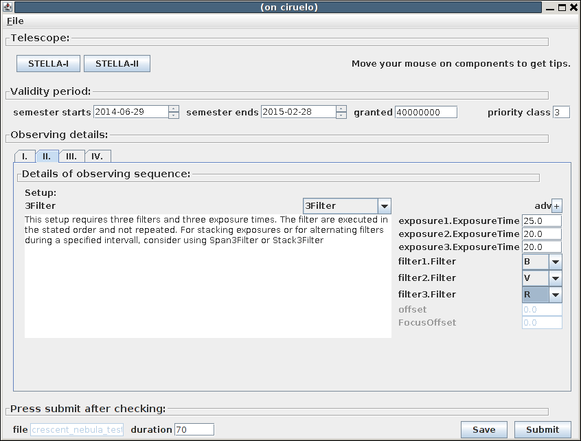
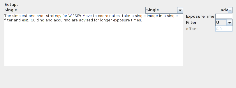
The next tab takes you to the details of the observing sequence. Normally, the Setup [5] is already pre-selected, depending on the observing sequence, you may specify an ExposureTime, plus the accompanying Filter [6] . Times are normally measured in seconds, angles in degrees, but rest your mouse pointer on top of the field to get some additional information on that particular format. Fields grayed-out are advanced setup possibilities. They can be activated with the adv+ [7] button. In the example shown, the advanced setup allows for a derotator offset [8] , in degrees, counted counter-clockwise, North up. Focus offset [9] is an offset afflicted to the current optimal focus position. It is stated in mm. For a description of the supported setups see Supported setups.
Target preparation tool, setup (2nd) tab
Footnotes
| [5] | The setup defines the filter plus the respective exposure times, it may contain information on dithering and number of exposures per single execution. |
| [6] | On the imager, on of the Johnson/Stromgren/Sloan set plus Hα wide/narrow. No filter (=clear) is also possible. |
| [7] | Clicking this button allows adjustment of the advanced features, only intended for experienced users. |
| [8] | The derotator offset in degrees. Cannot be chosen if off-axis guiding (see next page) is selected. |
| [9] | After deriving the best focus position (either from the ambient temperature or by executing a focus sequence), this offset is applied to the attained focus position. Negative values are intra-focal. |
Target coordinates and CCD read-out size
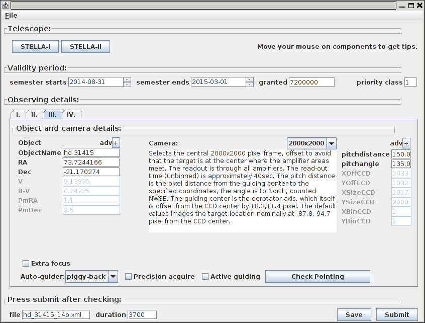
Here you enter the target coordinates. If you pick an ObjectName that is Simbad-resolvable, hit ‘enter’ after you filling out the field and wait for the data retrieval. Alternatively, you can specify RA and Dec (2000.0) either in natural units, i.e., degrees, or you might enter RA and Dec in sexagesimal format, using colons as separator chars, i.e., 4:54:53.86 for the right ascension. For the spectrograph, the V magnitude is also required. B-V and proper motions are used if stated.
To ease the selection of the read-out window, a few standard setups are provided in the Camera section. To avoid that your target object is exactely on the amplifier edges, a pitchdistance and pitchangle [10] are pre-defined. With the advanced settings, different geometries might be achievable. Note the two-amplifier readout on the the CCD version 2, implying an x-size of only half the required size. The window offsets [11] are in pixel from the upper-left corner. The entire chip is 4100x4100 pixel (including some ovserscan).
Both telescopes are equipped with a piggy-back guider scope. The Extra focus, if tagged, issues a focus sequence prior to the science exposure. The time accounts to the user’s granted total allowance and amounts to an extra time of typically 50 seconds. Check pointing allows the user to verify the pointing on the imager and the detection of close bright twin on the spectrograph. See How to gurantee guiding for details.
Target preparation tool, coordinates (3rd) tab
Footnotes
| [10] | To avoid your target to lie exactly an an amplifier edge. Not applicable for off-axis guiding, there RA & dec have to be adjusted. |
| [11] | Non-central window only possible in y-direction. |
Scheduling preferences and hard constraints:
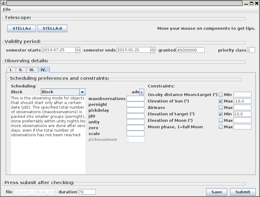
This is the section where you enter the constraints when your target should be picked within its validity period. Normally, the Scheduling type [12] is already preselected. Depending on the type, various other selection criteria have to be added. Hoover with your mous pointer on the fields to get additional information on the meaning and unit of the required information. A list of all scheduling modes can be found here.
The Constraints may be selected at will, elevation of target and Sun have some pre-selected values, which can be altered, of course. Any constraint must be satisfied during the entire duration of the observation, as estimated in the duration field. If the target just fails slightly, it won’t be picked at all. This has to be considered especially in cases, where you want rather continuous observation of your target for, e.g., six hours. Even if already one constraint (particulary dangerous are Elevation of Sun or Elevation of target ) is violated within the example six hours, your target will not be picked, even if it has otherwise perfectly high priority.
Target preparation tool, scheduling (4th) tab
Footnotes
| [12] | The scheduling mode is determined from your proposal, making a particular precise description of the observing plan mandatory. |
Supported setups
WiFSIP (Imager) on STELLA-I
Single exposure
3Filter
Predefined single-execution templates are provided for up to three filters. Specify exposure time and filter for each. If more than three filters are needed, use FullFilters.
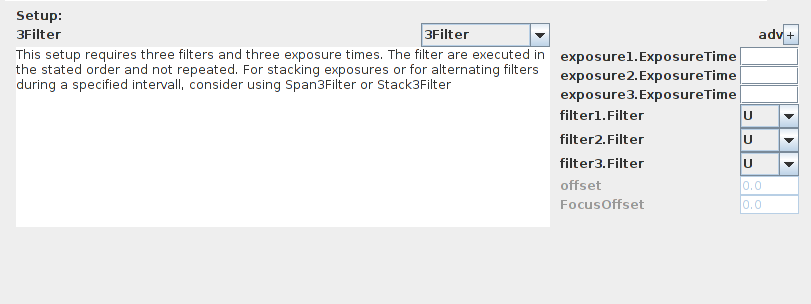
3 filter setup
Multiple exposure
Stacking
This is the simplest case of a multi-exposure setup. You state a single exposure time in seconds plus a number of repetitions. All exposures are done in the same filter.
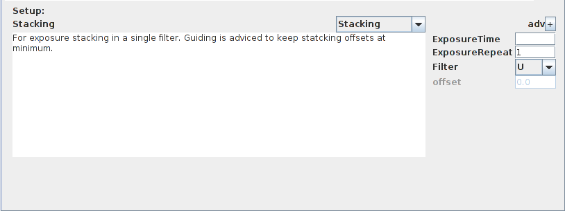
Stacking setup
5FilterStack
Predefined stacking sequences are available for at most five filters. This is shown here. Specify the five exposure times and filters separately, the repetition counter counts the number of blocks, i.e., 10 would mean a total of 50 exposures here.

5 filter stack setup
FullFilters
This setup allows total control of the filter sequence. Start with defining a single main exposure time (10 sec. in the example). Then, issue the total number of exposures, not the number of repetitions of the sequences in the next field (16 exposures in the example). The filter sequence and the exposure increase specify the filter to use plus an individual multiplication factor for the principal exposure time. In the example, five exposures in V at 20 sec. will be followed by three exposures in B, 30 sec. each. Note that you have to spell the filter names correctly, otherwise execution will fail at run-time. The available filters are: clear; U,B,V,R,I; u,v,b,y,hbw,hbn; up,gp,rp,ip,zp; haw,han.
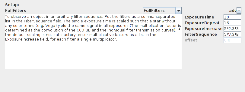
Full filter setup
Predefined time coverage
If you want to cover a target for certain time spans (e.g. eclipses), making as much exposures as possible, these are the setups you can use.
Span
The simplest case: Define an exposure time and a single filter, repeat for SpanSec seconds. Depending on the chosen exposure time and the requested read-out size this will result in a certain number of exposures n<SpanSec/ExposureTime.
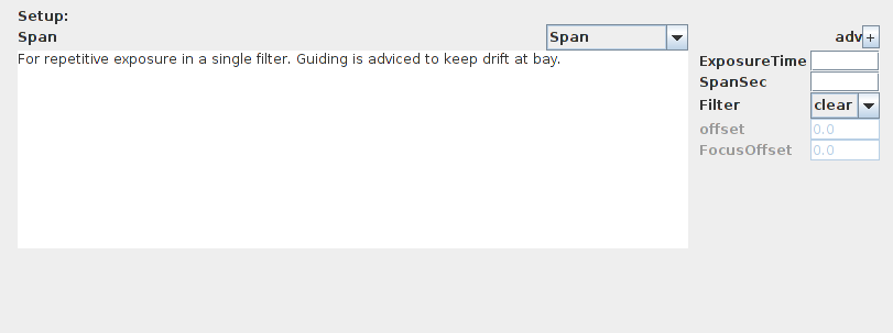
Span setup
5FilterSpan
Predefined sequences are available for at most five filters. This is shown here. Specify the five exposure times and filters separately, the cycle will repeat until the specified maximum span is reached. If within a cycle, the cycle will be continued until finished.
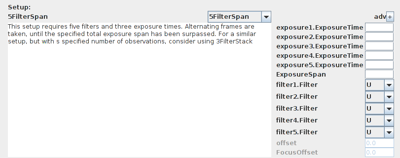
5 filter span setup
Dithering
Dithering is currently only available for piggy-back guiding, not for off-axis guiding.
RandomDither
This sequence needs only a dither offset as an arcsec-pair in α and δ. The actual dither applied is randomized at run-time, distributed Gaussian with a σ as specified. In total, Count images are taken.
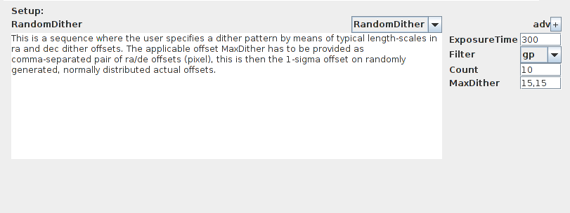
Random dither setup
SpiralDither
Gives the user total control on the applied dither pattern. The dither has to be supplied in pairs of α and δ dithers, separated by a semicolon. If less then Count pairs are supplied, the pattern is repeated.
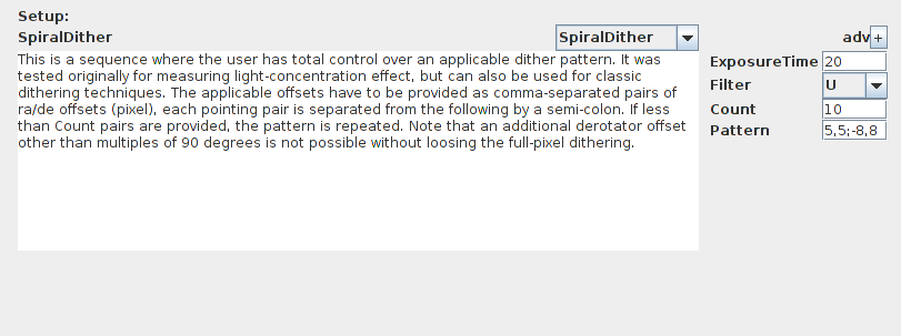
Spiral dither setup
Dither2Filter
Currently, only dithering with a maximum of two filters is supported. Within this setup, the provided dithering is applied at the start of each two-filter block, i.e., in the example a B and a V exposure is done at offset 0,0 to α and δ, then an offset of 5 and 5 arcsec is applied, and again a B and a V exposure are taken.
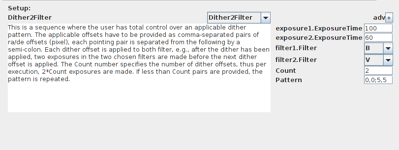
Dither 2 Filter setup
SES (Spectrograph) at STELLA-II
On the spectrograph, only two setups are currently available.
Spectrum
Takes a single exposure with the stated exposure time. Consult the ETC to get a S/N estimate.
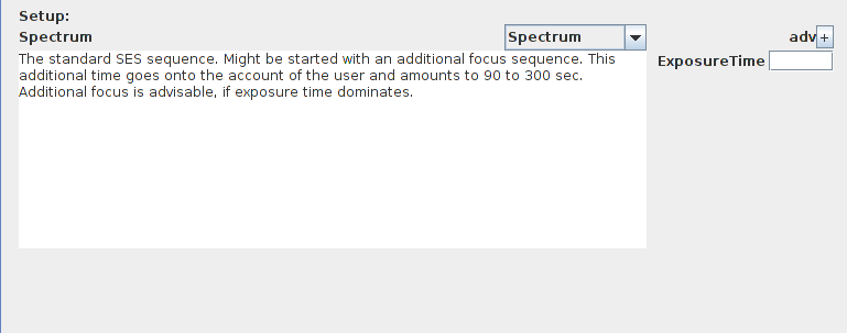
Spectrum setup
Stacking
Takes the number of requested exposures immediately after one another. The exposure time is the exposure time of a single exposure.
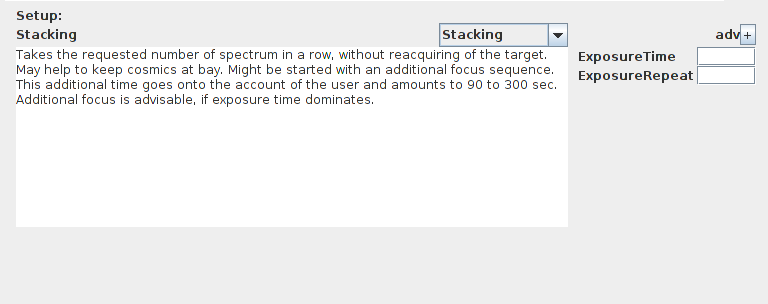
Spectrum stacking setup
How to gurantee guiding
Both telescopes are equipped with auxiliary refracting telescopes, mounted piggy-back on the main telescope. The are used for first checks of the telescope’s pointing. The spectrograph (SES) uses a fiber-viewing camera, which is used for fine acquisition and guiding. It cannot be de-selected. The imaging telescope, though, features an off-axis guider whit a very limited field of view, but mounted within the (derotated) instrument flange, thus picking a rather big annulus out of the available sky. If the user selects the off-axis guiding mechanism, the check pointing button changes to a default guide star close to this annulus.

Automatic guide star selection
Be warned that the automatic method tries to select a bright star (for best guiding cadence), at the expense of derotator setting. It might even be necessarry to shift the pointing center slightly. To change the selection, press the button.
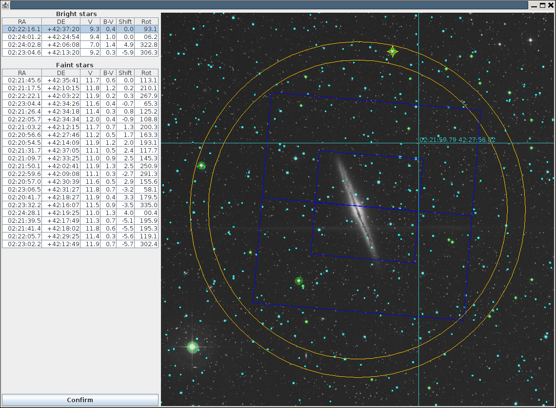
Interactive off-axis guide star selection
In the pop-up window, you see the annulus (orange) around the α δ you entered, overlayed on a DSS image. The blue outline is the current chip orientation plus read-out size, if non-full areas have been selected. The currently active off-axis guide star is marked in yellow. Stars considered bright enough for full cadence are marked with green double-circles, faint guiding stars, which require exposure times above the optimal cadence time, but still bright enough to be used for guiding are marked with single green circles. Move around in the Table or click on the star to change the selection. Leave the window by pressing confirm.
If you just want to check the DSS around your target star, e.g., for detecting bright binaries that might mess up the proper identification of your spectrographic target, use check pointing. The orange annulus in SES is the field-of-view of the fiber-viewing camera, the inner area denoting the area always visible on the fiber-viewing camera, the outer depicting the outer edge of the possibly visible area (depends on parallactic angle). The target star is marked in yellow. All the stars found in the catalog are surrounded by cyan-colored boxes. The case shown to the left is YY Gem, which has a very bright companion: Pollux, β Gem. Note also that your target may not be properly identifiable, if bright stars within the field-of-view of the fiber viewing camera are missing. In the latter case, they can be added manually to the target XML file.
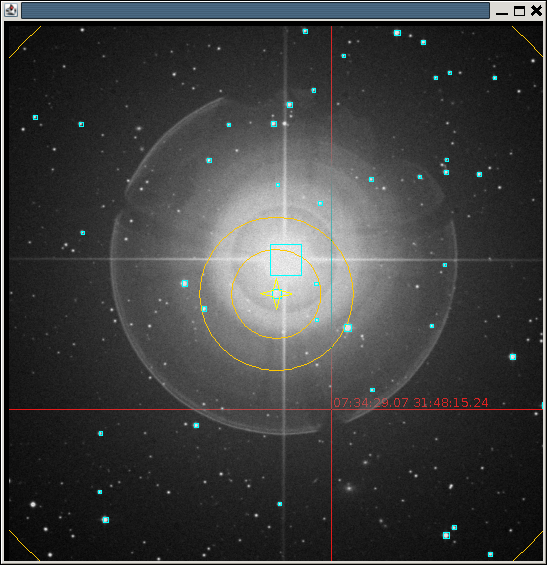
Checking the Field-of-view for SES (example: YY Gem)